How I learned to stop worrying and love the Free Energy Principle
In my lab, we’ve been thinking a lot about how the brain learns a model of the world and how it uses it to act intelligently. This seems to be the crux of intelligence.
How do brains do this? If we understood this completely, we could build a brain. A brain like ours. That would be pretty cool. At that point, I’d have to close up shop and move on to some other research direction. Interestingly, out of all the theories in neuroscience, very few could ever be used to actually build a brain – and most don’t even pretend they could! However, there is one that at least claims to. It’s called the Free Energy Principle. If you haven’t heard of it, you should watch this nice animated youtube short that introduces it quite well.
The Free Energy Principle (FEP) is a so-called “general theory” and a lot of neuroscientists I know don’t like it. There are two main types of criticisms I’ve heard: Either people can’t make any sense of it, or it’s “unfalsifiable” and they aren’t sure if it is any more useful than Bayesian inference or some more familiar theory.
This blog post is meant to be a gentle introduction to the math behind the FEP. We’re going to start really simple and find that it stays pretty simple, but it gives us nice mathematical quantities for talking about concepts we are interested in. In the same way that Bayesian inference has been a powerful tool for formalizing certain perceptual phenomena, FEP provides a few additional quantities that are useful for talking about what brains do. Moreover, we’re going to find that one quantity, the KL Divergence, is at the heart of it all. For a related (and genuinely more thoughtful) post, check out Hadi’s blog here. Finally, we’re going to stop short of active inference here and punt entirely on action. I’ll revisit that in a future blog post, but this will remain a good primer for that.
Note: The title here is a reference to a dark comedy from the height of the cold war called “Dr. Strangelove Or: how I learned to stop worrying and love the bomb”. I haven’t seen the movie since I was a kid, and I don’t remember anything except the line “not only is it possible. it is essential.” and that’s how I now feel about the KL Divergence.
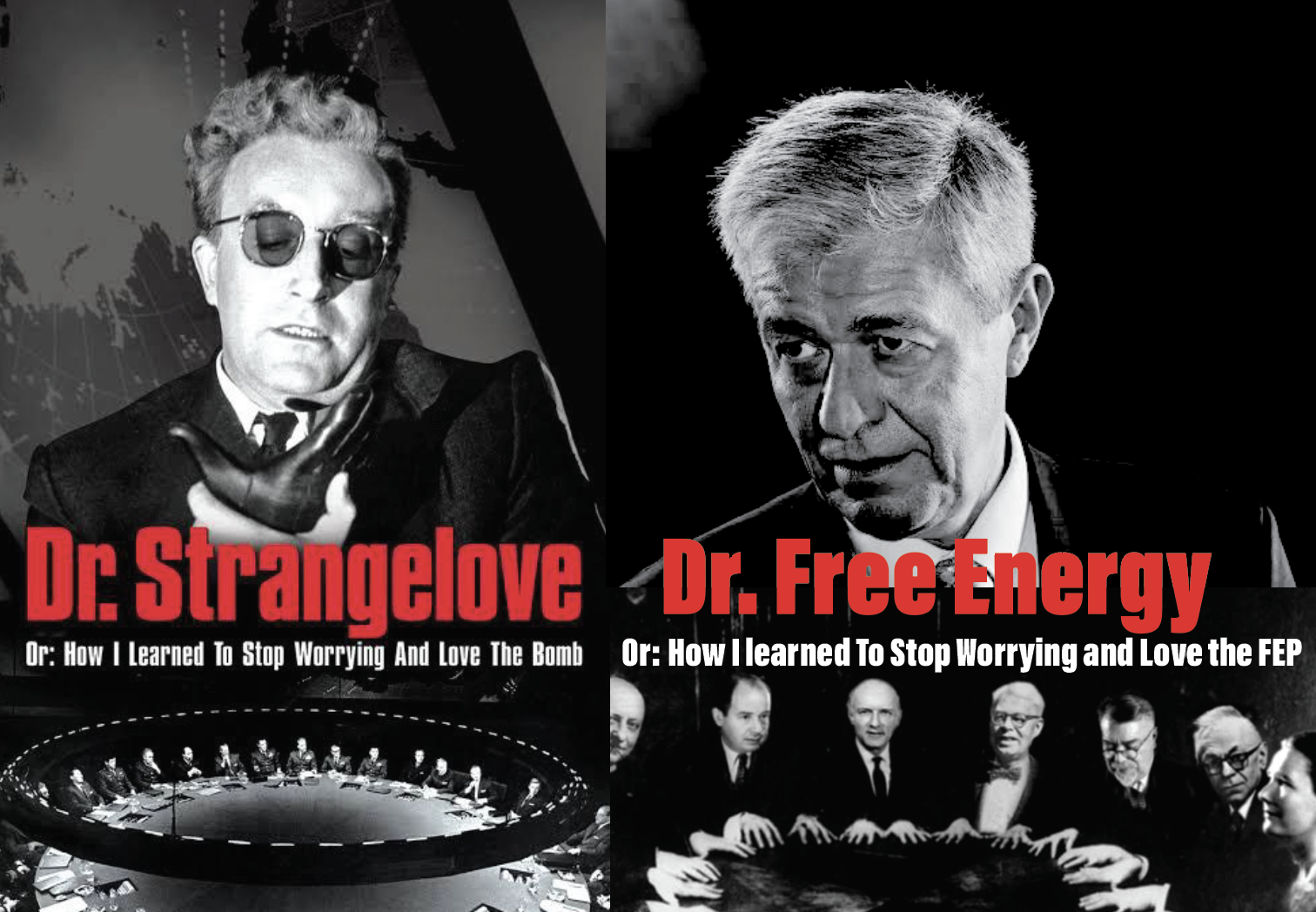
Left is the original movie poster. Right is the new and modified Dr. Free Energy, or: how I learned to stop worrying and love the Free Energy Principle. Karl Friston on top, and the "cybernetics seance" from the Macy conference (with Norbert Weiner, John von Neumann, Walter Pitts, Margaret Mead and others) on the bottom.
The problem
Let’s start out with some solid ground: there IS a world out there. And the brain just gets samples from it through the senses. I’m going to massively over-simplify the problem in this blog post (don’t worry, it still works even if we don’t do this), but let’s pretend the brain is passive and only receives sensory samples, .
is the true generating processs of the world for our passive brain. The brain does not have access the true generating process, , and so it cannot evaluate the density even though it can get samples from it. For now, we’re going to assume sammples are i.i.d. (ignoring actions/dynamics). That is a very incorrect assumption for brains, but it makes the math easier, so we’re going to stick with it for now to gain some intuitions.
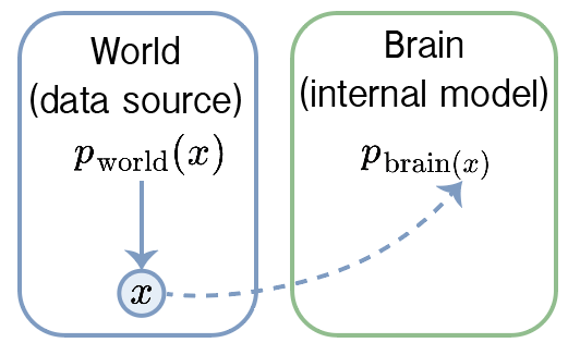
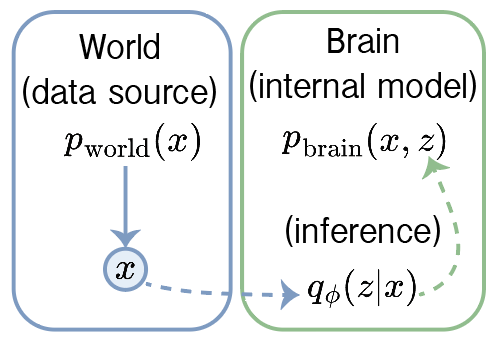
The world generates data. The brain can only sample this data and must adjust its own internal model to match. In all cases, the brain can only evaluate its own model density p_brain.
I’m going to be careful to keep track of what is in the world and what is in the brain, and will keep the notation clear. The brain can’t evaluate , because that’s literally the physics of the world, but it can evaluate its own model of it for any . Let’s say the brain’s model has parameters, , so we write it as . How do you fit a good to given only samples? That’s what we’re going to solve here.
What follows is a simple walkthrough in notation that I like, but is unusual in the active inference literature. I think you’ll find that the math lends itself quite nicely to talking about what the brain is doing.
Setup
This section lays out all the math facts that you need for all the derivations that come.
1) Log-likelihood
Suppose we have the brain’s model, , and i.i.d. samples from the world, . The likelihood is just the probability density evaluated at the observed data combined across all samples:
Given fixed data, the likelihood is a function of the parameters . The reason we can multiply them all together is the i.i.d. assumption I made above. Because multiplying many small numbers quickly becomes impractical, we usually work with the log-likelihood, here the average log-likelihood or per-sample log-likelihood:
Intuition
Think of the log-likelihood as a surprise meter with the sign flipped. If your model assigns high probability to what actually happened, the log-likelihood is high; if it assigns low probability, the log-likelihood is very negative. So if an improbable event happens, your negative log-likelihood spikes positive. Therefore, minimizing the negative log-likelihood, or equivalently, maximizing the log-likelihood, is just trying to reduce your surprise across many observations.
2) Expectations and the Law of Large Numbers
An Expectation is the average quantity you would get from many draws under the data-generating law, . The expectation of a function is
If , then by the law of large numbers
If we apply this to our per-sample log-likelihood above, we get:
Intuition: averaging samples from weights values by how often they occur. Points with larger show up more and pull the average toward them, so the average of log-likelihood of the samples is a weighted average (weighted by ) and converges to the expectation with enough samples.
Importantly: the expectation is w.r.t. , the true generating process of the data. Our model log likelihood is evaluating , but it’s evaluated at samples from .
3) KL divergence
The Kullback–Leibler (KL) divergence will emerge as a quantity of major interest. Here, I’m going to introduce it using it’s definition, but I really want to emphasize that it emerges in the derivation below. I want to define it here so we’re prepared to recognize it when it shows up, so we can interpret it accordingly. The KL divergence measures the mismatch between two distributions — in this case, the true world distribution and the brain’s model . Its definition is:
Intuition: KL as an expected log-likelihood ratio
Let’s go back to basic statistics. For a single sample , we know how to compare two models, and : we use the log-likelihood ratio: . If we had many samples, we would average the log-likelihood ratio across all samples. With a large enough number of samples, the average converges to the expectation (that’s just point 2 above).
Now, what happens if we’re sampling from and then evaluating the log-likelihood ratio compared to ? Well, then we get the KL divergence! It’s an expected log-likelihood ratio when you’re sampling from the first density. It’s bounded at . It has to be positive. And what it tell us is how much extra “surprise” we get when we use (the wrong model) to explain data generated by .
For our problem, if the brain’s internal model matches the world perfectly, the KL is 0 — no extra surprise. But the more the brain’s predictions diverge from the world’s samples, the larger the KL becomes. In other words, KL measures the cost of pretending the brain’s model generated the data when in fact it came from the world. This is exactly what we want to minimize. Small KL is the mathematical equivelent of saying the “the brain’s model fits the world well”.
Properties worth knowing
- , and it’s 0 iff .
- It’s asymmetric: .
- Connection to cross-entropy:
where is the cross-entropy.
Maximum likelihood is KL minimization
Given fixed data, the log-likelihood is a function of the model parameters , and all it tells you is the log probability of each sample. If we maximize the log-likelihood (or equivalently, minimize the negative log-likelihood), what happens? This is a classic technique in statistics called maximum likelihood estimation, and we’re going to walk through a visual example of what it looks like when the average log-likelihood is maximized.
Below is a simple example with a true generating distribution that is a 2D Gaussian. The data, , are shown in red. Our model is also a 2D Gaussian and is shown in blue. The model, , with parameters . Withough knowing the true parameters, we can evaluate the average log-likelihood of the data under our model, and we can adjust our parameters to maximize this quantity by stepping along the derivative with respect to the parameters. At first, our model is not overlapping with the data. You can hit “Run Optimization” to see what happens if we simply step along the gradient (derivative) of the log-likelihood.
Data Points & Model Distribution
Average Log-Likelihood vs Steps
It’s fun to watch the animation, and is a totally standard method in statistics. But did you ever stop to ask why this works? Why does assigning high probability to likely samples make our model fit the true generating distribution?
What is happening when we maximize likelihood? Or, equivalently, when we minimize negative log-likelihood?
Let’s rearrange some terms using the fun facts from above and see what happens. With enough samples, we can use point 2 above. With a large number of samples, the average negative log-likelihood converges to the expected negative log-likelihood (NLL) under the true world distribution:
Make it equal to itself and add and subtract :
Now we can combine the first two terms using the log rule :
And then split the expectation and simply recognize the KL divergence and the entropy of the world:
So there you have it. We started with the average log-likelihood and rerranged the terms and it revealed that minimizing the negative log-likelihood is equivalent to minimizing the KL divergence between the world and the brain’s model.
The first term (entropy of the world) does not depend on . Therefore, minimizing expected NLL is the same as minimizing the KL divergence between and !
That simple result is satisfying: Maximizing likelihood makes the brain’s model assign high probability to what the world actually produces AND it tunes to get as close as possible to . This intuition helps unpack Alex Alemi’s wonderful blog post on KL divergences and how central they are. Maximum likelihood is just a special case of KL minimization. Additionally, this is not true for any arbitrary distance metric or divergence. As far as I know, the KL divergence has a priveleged status.

Hidden causes: the brain’s internal variables
So far we treated the brain’s model as a direct mapping from observations to probabilities, . That’s too simple, because the brain needs to be able to flexibly encode the state of the world in terms of hidden causes. Let’s call these hidden causes . Importantly, these are not the “real” physical causes; they’re useful internal variables the brain uses to understand the world.
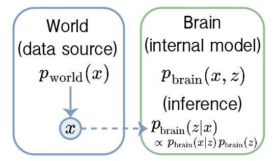
All samples of data come from the true generating process p_world. The brain wants to explain these samples using a generative model with hidden causes, z. The brain can only sample from p_world, but it does not evaluate it. To fit the data well, it must adjust the parameters of its internal model as well as infer the latent causes. Importantly all these causes are in the brain NOT the world. The density that generates samples is the world. The densities used for inference are in the brain.
The brain’s model says: first sample a hidden cause from a prior, then generate an observation from a likelihood.
Here we have the static parameters of the brain , which could map onto the weights of a neural network (or the synapses in a brain). And we have the latent variables , which are the internal latent variables the brain uses to understand the world (which could map onto the activations or spikes of neurons).
Two things we want to do with this model:
- Learning (adapt the world’s statistics): make match as well as possible using samples .
- Inference (adapt to the sampled data): given an observation , infer its hidden causes via the posterior
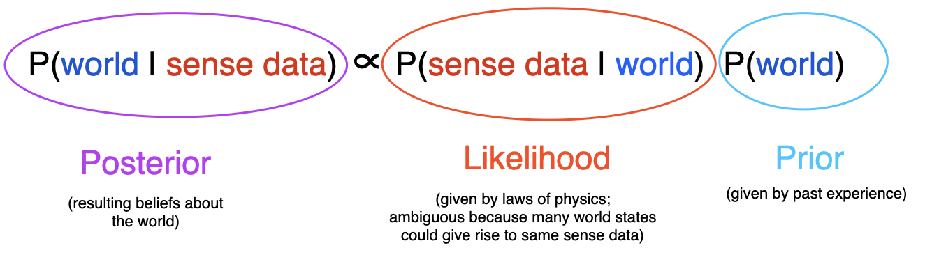
This is just Bayes rule and it maps nicely on to words we use to describe perception. But, I want to spend a moment to belabor a recurring issue in perceptual psychology.The way Bayesian inference is typically introduced in perception is that the brain is inferring the causes in “the world” from “the senses”.
In a typical Bayesian Brain experiment, psychologists and neuroscientists will test to see if the subject has behavior that looks like Bayesian inference over the parameters of their experiment. For example, they might show drifting motion where some motions are more likely than others and see if the subjectls learn to integrate the prior probabilities of the motion (in the experiment) with the incoming visual evidence.
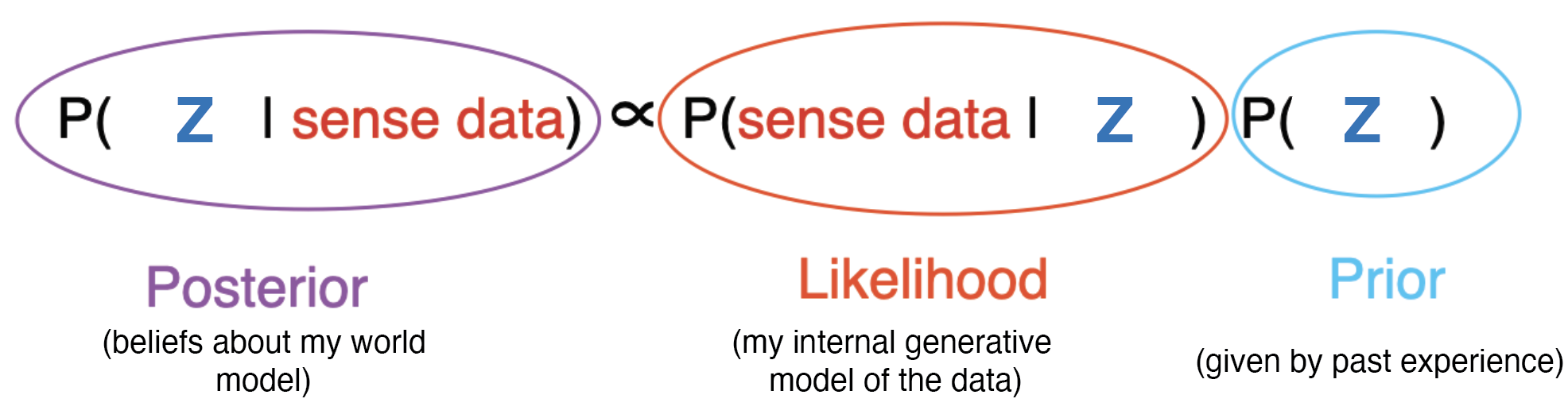
But that’s NOT what is happening here. are in . They are NOT in . The experiment is part of , but are not. To learn to act intelligently in the world, likely have high mutual information between relevant groundtruth causes in the world – the intuitive physics level, but no more. The key point is to remember that are not the “real” causes in the world (or your experiment). They are the brain’s internal representation of the world.
Now, even though are just causes that the brain made up, that denominator is still usually intractable, which makes the exact posterior intractable too.
We’re going to get around this by inventing a density we can evaluate and just try to optimize the parameters for that. We just invent a density we can evaluate, . Is this even reasonable? In the next section we’ll see that it is and why it works is quite satisfying.
The world still generates data. All samples come from p_world. The brain wants to learn the hidden causes in its generative model of the data. Again, it can only sample from p_world, but it does not evaluate it and z all live in p_brain. The brain adjusts its parameters, theta, and infers the latent causes, z. To do this, it uses a variational approximation to the true posterior. This is a distribution it knows how to evaluate and avoides the intractable integral.
Deriving the Evidence Lower Bound (a.k.a. Free Energy)
To get around the intractable posterior, we just invent a density we can evaluate, . This is the backbone of variational inference, and what we’re going to do here is derive a quantity known in machine learning as the Evidence Lower Bound (ELBO). The ELBO is typically derived using something called Jensen’s inequality, so I’ll show that first, but then we’ll do it without it to see what we were missing.
With Jensen’s inequality (lower bound)
Jensen’s inequality Jensen’s inequality says that the average of a logarithm is always less than (or equal to) the logarithm of the average:
It’s often explained in terms related to concavity, but if you think about the shape of the logarithm, it’s pretty intuitive. The logarithm is compressive for large values and explosive near zero, so a few tiny values pull the average of logs way down. If you average first, those tiny values are cushioned before taking the log.
Here’s the derivation you see in most places: Start from the model evidence:
Apply Jensen’s inequality (log of an expectation ≥ expectation of the log):
And we’re done! Call that thing the ELBO:
Importantly, the (variational) Free Energy is :
There you go! It’s not that mystical how to get there. But what is it good for?
Well, we can see from the inequality that it’s a bound on the “model evidence”… what we were calling log-likelihood at the top,
But what disappeared in that inequality? What are we actually doing when we minimize Free Energy?
Let’s rederive without Jensen and see what we’re missing.
Without Jensen (the exact identity)
Start with any tractable density (whose integral is 1):
What does this mean?
Well, now we can see clearly what disappeared in the Jensen’s inequality derivation: the KL divergence between the approximate posterior and the true posterior. This is not a bound anymore. It’s an exact identity. Now, because the KL is always , if we maximize ELBO using the varational posterior parameters , we are guaranteed to minimize the KL divergence between the approximate posterior and the true posterior. If we maximize ELBO using the model parameters , we can push up the model evidence and mimimize the KL between the world and the brain’s model. Thus, maximizing ELBO or minimizing Free Energy minimizing is particularly useful during inference for minimizing the KL between the variational posterior and the true posterior.
Putting it all together: What about learning? How do we make the brain’s model match the world?
So far we showed that maximum likelihood can be interpreted as minimizing the KL divergence between the world and the brain’s model. We also showed that minimizing Free Energy is equivalent to minimizing the KL divergence between the variational posterior and the true posterior. Now we’re going to combine them both to see what minimizing Free Energy is really doing.
First, remember that Free Energy is the negative ELBO:
Second, remember our trick up above that minimizing the negative log-likelihood is the same as minimizing the KL divergence between the world and the brain’s model:
Let’s put these together and see what happens when we minimize the Free Energy:
Conclusion (what minimizing Free Energy does):
- Improves the generative model (minimizes ).
- Improves inference (minimizes the expected ).
- The world’s entropy is constant in and — you can’t change physics; you can only make your brain model and inference better.
Conclusion
In this blog post, we derived the free energy principle from first principles. We learned that simply trying to assign high probability to probable events is equivalent to making the brain’s model fit the world well (by minimizing KL divergence). We learned that the Evidence Lower Bound (ELBO) is pretty easy to derive, even without Jensen’s inequality and that it leads to an exact identity rather than a bound, where maximizing ELBO is actually minimizing two intractable KLs that we’re really interested in minimizing. The KL Divergence emerges as a metric of how good our models are in two places. The KL between the world and the brain’s model tells us how well the brain’s model fits the world (Learning). The KL between the variational posterior and the true posterior tells us how well the brain’s inference matches the true posterior (Inference). Minimizing Free Energy is equivalent to minimizing both of these KLS! And the KL is really the mother principle!