Are photoreceptors doing predictive coding?

Are photoreceptors doing inference?

What a bizarre proposition! The photoreceptors (rods and cones) are the light-sensing cells in the retina. Despite their relatively simple function, they have the tough task of encoding many log-orders of luminance with a limited dynamic range. Therefore, they adapt both their gain and their kinematics as a function of the recent luminance. Many decades of work have gone into identifying a good functional model of the cones, with a relatively thorough biophysical model of the cones published only recently.

Here, I’m going to explore the possibility that the cones themselves are actually doing inference over a generative model of luminance. What would that look like? Let’s walk through that here.

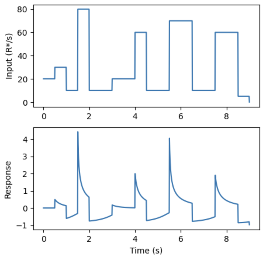
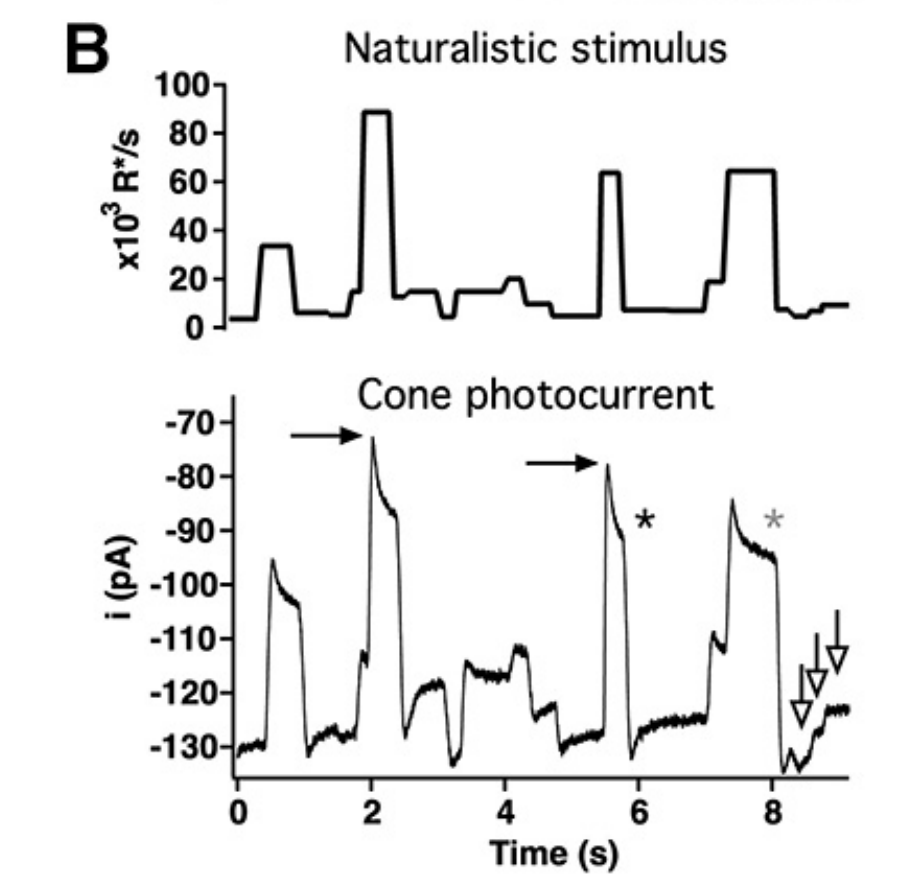
Before we start, let’s look at how real cones respond to realistic input.

Inference over a Generative Model of Temporal Luminance Signals

Let’s consider generative models of the form $p(I|\theta )$, where $\theta$ represents the parameters of the distribution and $I$ is the luminance signal.

So, to restate the problem, if I’m a cone, I want to estimate the paramters $p(\theta |I)$. There are a number of ways we could approach this, but this posterior probability will be intractable because of the normalization constant. Here’s an intuition for that: I’ve seen some light, but to estimate this posterior I need to know the probability of all possible luminance signals, which I can’t know (there might be some light I just can’t imagine).

There are two obvious ways around this, and as you’ll see below, they both lead to the same answer. The first is simply to use the derivative of the likelihood with respect to the parameters (a.k.a. the score function). The second is variational free energy minimization. You’ll see in a minute that under certain assumptions, these two methods are equivalent.

Free Energy Minimization

Let’s start with Free Energy minimization. This is the mathematical quantity in Karl Fristons Grand Unified Theory of life. And it’s a pretty general starting point. It makes sense somehwere else to derive it, but here I’m just going to jump in and start with the definition. The variational Free Energy is defined as:

$\mathcal{F}[q]={\mathbb{E}}_q[\log q(\theta )-\log p(\theta ,I)]$

What is $q(\theta )$? It’s a distribution we just get to make up over the parameters. Since we don’t know the true posterior, we’re just going to make one up. Now, what we’d like to do is minimize the KL divergence between our approximate distrubtion $q(\theta )$ and the true posterior $p(\theta |I)$. Free Energy minimization is a way to do that without touching $p(\theta |I)$ and it forms ais a lower bound on the log-likelihood of the data. We can rewrite the Free Energy into two terms as follows:

$\mathcal{F}[q]=-{\mathbb{E}}_q[\log p(I|\theta )]+\text{KL}(q(\theta )||p(\theta ))$

There are many good blog posts on why this quantity is a reasonable thing to minimize, but here the key point is that there are three distributions we need to choose: $q(\theta )$, $p(\theta )$, and $p(I|\theta )$. Let’s start with $q(\theta )$. One of the simplest things we can choose is a delta posterior $q(\theta )=\delta (\theta -{\theta }_t)$, which is a point mass at the current estimate of the parameters. If we assume a delta posterior, several important simplifications occur:

1. The expectation ${\mathbb{E}}_q[f(\theta )]$ of any function $f(\theta )$ simplifies to $f({\theta }_t)$
2. The KL divergence term $\text{KL}(q(\theta )||p(\theta ))$ simplifies to $-\log p({\theta }_t)$ for $p({\theta }_t)>0$

Substituting the delta posterior into the Free Energy and assuming $p({\theta }_t)>0$ we get:

$\mathcal{F}[\delta (\theta -{\theta }_t)]=-\log p(I|{\theta }_t)+\text{KL}(\delta (\theta -{\theta }_t)||p(\theta ))=-\log p(I|{\theta }_t)-\log p({\theta }_t)=-\log p(I,{\theta }_t)$

If we further assume a uniform (or flat) prior $p(\theta )\propto \text{constant}$, then:

$\mathcal{F}=-\log p(I|{\theta }_t)+\text{constant}$

So if we want to minimize Free Energy, we can simply step along the gradient of negative log-likelihood w.r.t. the parameters, which is exactly the score function.

So, why did I bother with all that if I’m just going to maximize the likelihood? Because we could have chosen different distributions and ended somewhere else, and that’s interesting. Free Energy minimization is incredibly flexible, but its worth understanding that it can reduce to familiar things like maximum-likelihood.

In the next section I’ll walk through a simple example with Gaussian distributed luminance, and then I’ll move onto a more physically realistic model.

Gaussian Luminance Model

Okay, let’s say the temporal luminance signal $I(t)$ is drawn from a Gaussian distribution: $I(t)\sim \mathcal{N}(\mu (t),{\sigma }^2(t))$

The probability density function is:

$p(I|\mu ,\sigma )=\frac{1}{\sqrt{2\pi {\sigma }^2}}\exp \left(-\frac{(I-\mu {)}^2}{2{\sigma }^2}\right)$

and the log of that is:

$\log p(I|\mu ,\sigma )=-\frac{1}{2}\log (2\pi )-\log (\sigma )-\frac{(I-\mu {)}^2}{2{\sigma }^2}$

The score function is the gradient of the log-likelihood with respect to the parameters. For $\mu$:

So, the update rule for $\mu$ is:

$\mu (t+1)=\mu (t)+\eta \frac{I(t)-\mu (t)}{{\sigma }^2(t)}$

Let’s repeat for $\sigma$. For numerical stability, let’s work with $\log (\sigma )$:

So, the update rule for $\log (\sigma )$ is:

$\log (\sigma (t+1))=\log (\sigma (t))+\eta \left[\frac{(I(t)-\mu (t){)}^2}{{\sigma }^2(t)}-1\right]$

so to get $\sigma (t+1)$ we can exponentiate both sides:

$\sigma (t+1)=\sigma (t)\exp \left[\eta \left(\frac{(I(t)-\mu (t){)}^2}{{\sigma }^2(t)}-1\right)\right]$

So that’s it, let’s assume our cones are doing inference over this generative model, and we’ll assume they’ll report something like the prediction error. In this case the score function for $\mu (t)$:

${\partial }_{\mu }\mathcal{F}=\frac{I(t)-\mu (t)}{{\sigma }^2(t)}$

What does this look like?

todo: have a figure

More realistic distributions

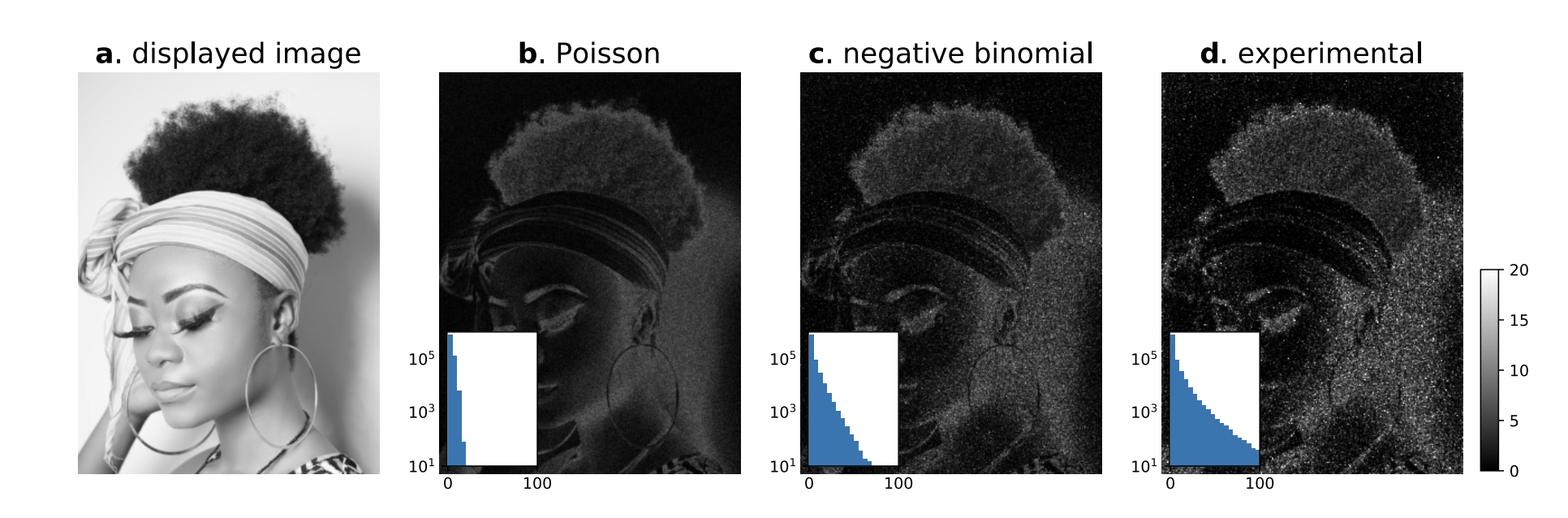
Light is not Gaussian. Let’s try to make a physically realistic distribution. Photons are poisson distributed given a fixed light level. If light levels are fluctuating locally at all (as they always do in the real world), then light will be a rate-modulated Poisson proces, captured by a Negative Binomial distribution.

Interestingly, my graduate student recently measured the noise in event cameras and found that negative binomial noise was a good approximation of the noise in static scenes measured with high frame rate event cameras

Negative Binomial Distribution Cones

The Negative Binomial distribution models count data with overdispersion. For our temporal luminance signal $I(t)$:

$I(t)\sim \text{NB}(\mu (t),r(t))$

Where $\mu$ is the mean and $r$ is the dispersion parameter. The variance is $\mu +\frac{{\mu }^2}{r}$.

The probability mass function is:

$p(I|\mu ,r)=\frac{\Gamma (I+r)}{\Gamma (I+1)\Gamma (r)}{\left(\frac{r}{r+\mu }\right)}^r{\left(\frac{\mu }{r+\mu }\right)}^I$

where $\Gamma$ is the gamma function.

The log-likelihood is:

The score function with respect to $\mu$ is:

and the score function with respect to $r$ is:

The gradient of negative Free Energy with respect to $\mu$ is what our cones will spit out:

$\frac{\partial \mathcal{F}}{\partial \mu }=\frac{I}{\mu }-\frac{I+r}{r+\mu }$

So what does this look like?