Generalization in data-driven models of primary visual cortex

This is entry is the first in a journal club series, where I do a deep dive into a paper I’ve recently gone over in a journal club or lab meeting.

Today we’re discussing Lurz et al., 2020 from Fabian Sinz and colleagues. In it, they introduce a few new tricks for fitting CNNs end-to-end to neural data. Then they show their data-driven model generalizes to predict the responses of neurons that it wasn’t trained on (in animals that were not part of the training set!)

The main points of interest for me were:

• General conceptualization of “readout” and “core”
• “Tricks” for learning the readout
• Generalization performance

“Readout” and “Core”

Many groups have now presented advantages to thinking of neural population activity as resulting from shared computations with neuron-specific weights. Rather than optimize a model that predicts the responses of each neuron, $r^{(i)}$, given the stimulus, $x$, assume that each neuron operates with an affine transformation (“readout”) of a core stimulus processing model that is shared by all neurons.

The simplest versions of this have a single linear filter as the core. For example, Batty et al., 2017 used knowledge of the cell class to group retinal ganglion cells and learn a single space-time linear filter for all neurons of the same class. Their “multitask LN” model has a single filter for all On-RGCs and each neuron simply scales that filter’s response with a neuron specific gain and offset term and then passes that through a sigmoid nonlinearity.

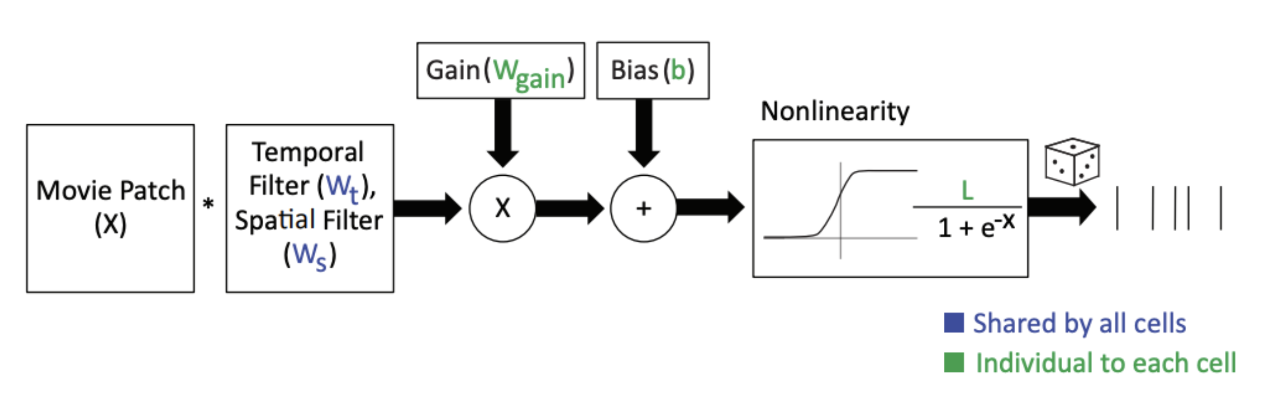
I really like the terms “core” and “readout” and think they should be adopted as the standard nomenclature for such a model. In the figure above, the blue parameters ($W_t$ and $W_s$) are shared by all On-RGCs and form the “core”. The green parameters form the “readout”.

In this case, the core is simple and interpretable (it’s a single space-time separable linear filter). The readout is also simple. It’s a gain and offset term per neuron. But this conceptual framing scales nicely to talking about much more complicated neural network models and nicely delineates their distinctions. But, every model consists of a “core” and a “readout”.

Two basic types of cores

Once you accept the “core” and “readout” distinction, cores have two basic distinctions in neuroscience research. They can either be “data-driven” or “goal-directed”.

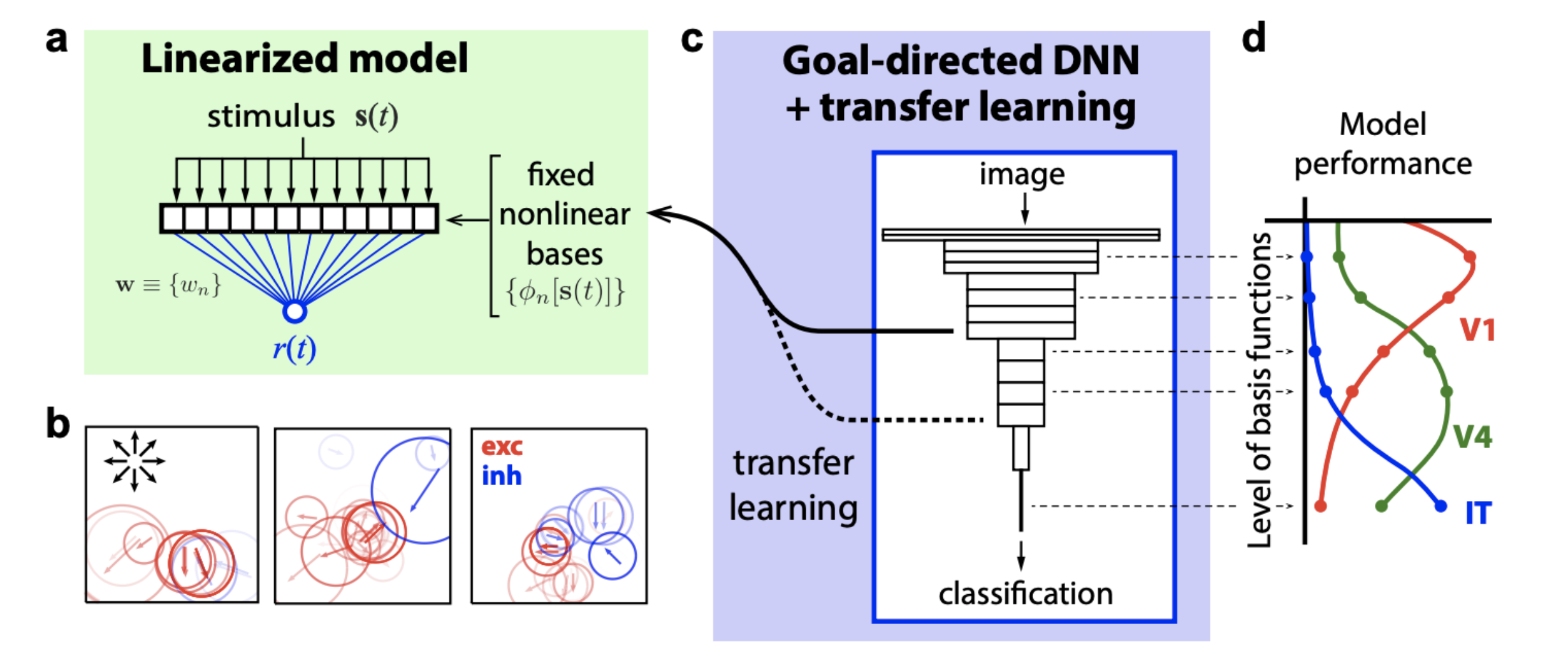
Goal-directed cores consist of a model that was trained to do some task given a stimulus (e.g., object classification). We’ve seen this successfully applied in neuroscience to a number cases, particularly in the ventral stream of primates (e.g., Yamins et al., ).

Data-driven cores learn the core directly from the neural activity.

This idea is really just something that has been said by others already (e.g., this paper from Dan Butts), but I’m converging on certain language for talking about it myself: “data-driven core” vs. “goal-directed core”.

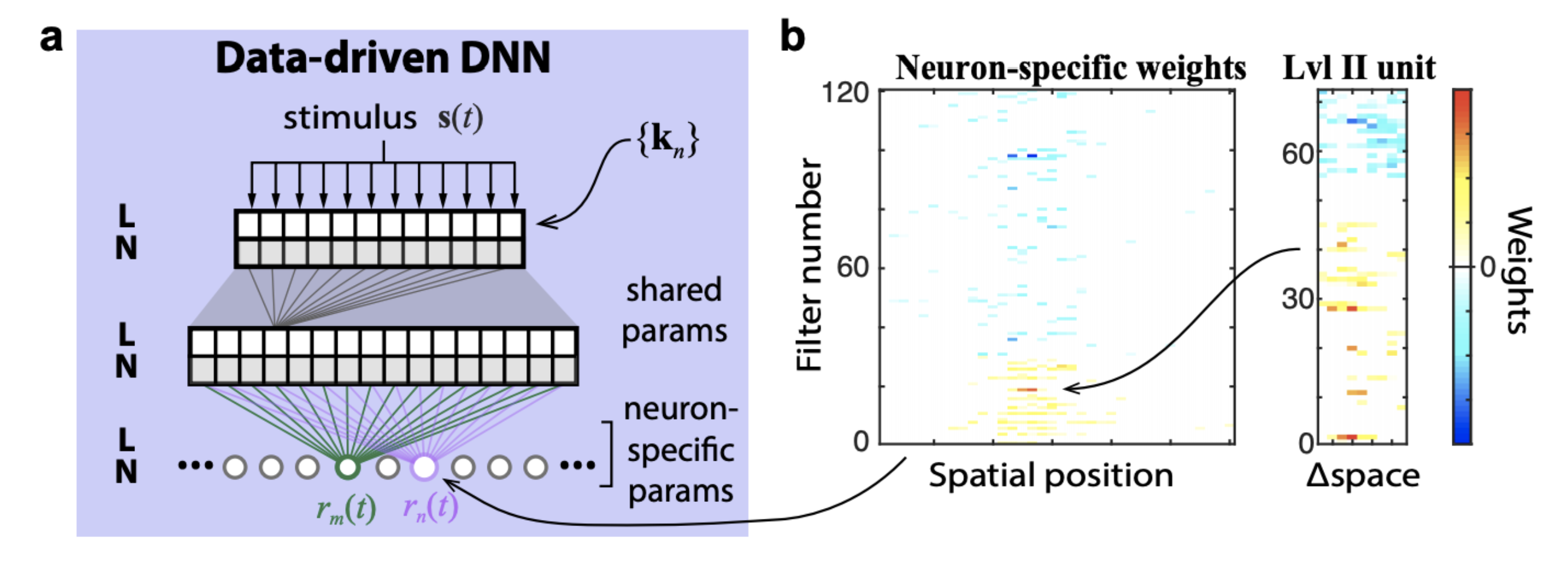
The figure below demonstrates the logic of a data-driven core. It is trained end-to-end from stimulus to spikes. The core is shared by all neurons and the readout is neuron specific.

In contrast, a goal-directed core comes pre-trained (on some other dataset) and and forms a nonlinear basis for a linearized model of the neural responses.

The advantages of a goal-directed core are:

1. they can use much more data than is typically available in a neural recording
2. they have an explicit task, so they provide convenient language for talking about what the core does

The advantages (hopes) of data-driven cores are:

1. they nonlinearities that are brain specific (opposed to input-specific or task-specific)
2. can be constrained with brain-inspired architecture

There are disadvantages to both approaches as well. The primary disadvantage of goal-directed cores in vision is that you’re mostly stuck with whatever the ML community has been most excited about. I think this has had an unfortunate side effect of pushing more of visual neuroscience into studying the responses to images (because that’s what the models can do). Of course, goal-directed cores can also be constrained with brain-like architecture and trained from scratch, and we’ll probably see more of that happening, but then you’re back dealing with data/computation limits. Another limitation of a goal-directed network is that you have to know what the neurons do a priori instead of just knowing what their inputs are. What does the retina do?

Okay. Now that we’re all on the same page, a real test of a data-driven core is whether it can generalize like goal-directed cores do. Goal-directed cores are generalize from the task they were trained to perform to predict neural activity by training the readout. Lurz and colleagues do the same thing here. Train the core and readout on one set of neurons, then fix the core and train only the readout on another set of neurons.

Old “Tricks” for learning the readout

For a typical convolutional neural network (CNN), the per-neuron readout scales with the size of the input and the number of channels. For example, the activations of the final layer of a CNN, $a=\text{F}[x]$, where $x$ is an image of size $w\times h$, is $a\in {\mathbb{R}}^{w\times h\times c}$ where $c$ is the number of channels in the network.

For the models the authors are considering here, the image size is $64\times 36$ so there are 2304 parameters per output channel per neuron! Even with structured regularization (smoothness, sparseness), this is a big problem to fit in a normal dataset.

There have been a series of “tricks” for learning the readout that these authors have rolled out over the last few years.

Trick #1: Factorized readout (Klindt,Ecker et al., 2016)

The first trick is to learn the same spatial readout for all channels in the model. This separates “what” features the neuron integrates from “where” the neurons are spatially selective.

The activations, $a$, are size $[N\times c\times w\times h]$, where $N$ is the batch size, $c$ is the channels, and $w\times h$ are the width and height of the input images. The activations are multiplied by a feature vector, $w^{(i)}\in {\mathbb{R}}^c$, and a spatial weight vector, $v^{(i)}\in {\mathbb{R}}^{w\times h}$, where $i$ is the neuron index.

Therefore the response of neuron $i$ will be

$r^{(i)}=F_i\left[{\sum }_{w,h,c}{w}_c^{(i)}{v}_{w,h}^{(i)}{a}_{c,w,h}\right]$

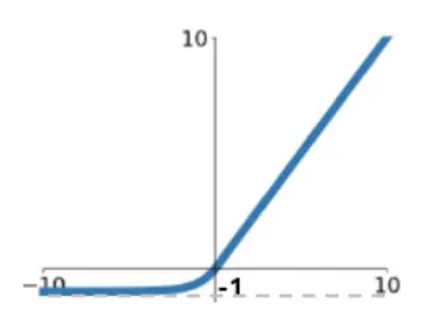
where $F_i$ is the activation function for neuron $i$, which is an ELU with an offset.

This reduces the number of parameters from $2304\times c$ to $2304+c$

Trick #2: coordinate readout using bilinear interpolation, learned with pooling steps (Sinz et al., 2018)

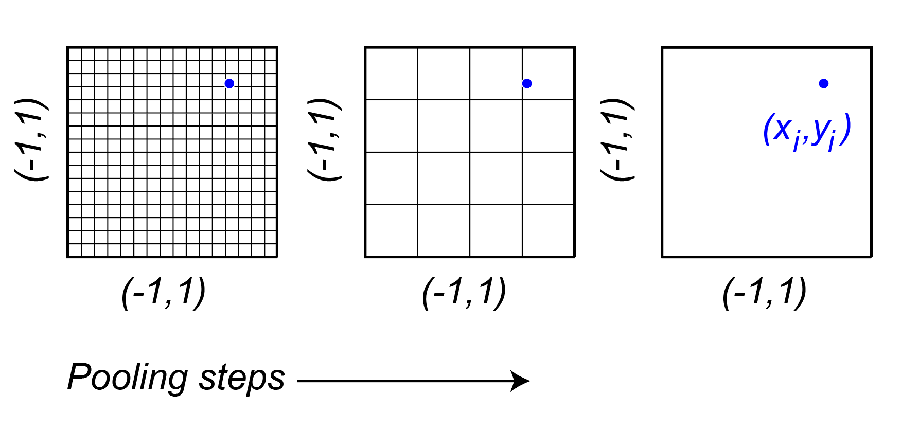
This approach assumes that each neuron has a feature vector that reads out from a spatial position (a single point) in the spatial output of the network.

The spatial position for each neuron, $x_i,y_i$ are learned parameters. They are sampled at sub-pixel resolution using bilinear interpolation. The issue with learning $x_i,y_i$ is that if the initialization is far away from the true retinotopic location of the neuron, then the gradients will be zero. To circumvent this, the authors represent the feature space of the core at multiple scales using $4$ average pooling steps with $4\times 4$ pooling with a stride of $4$, such that the final stage is a single pixel. They then learn a feature vector that combines across these scales. $x_i,y_i$ can be any value within a $1\times 1$ feature space and that way there are gradients to support the learning of the features and the position.

This readout idea comes from spatial transformer layers. The basic transform operation is an affine transform of a grid of sampling points.

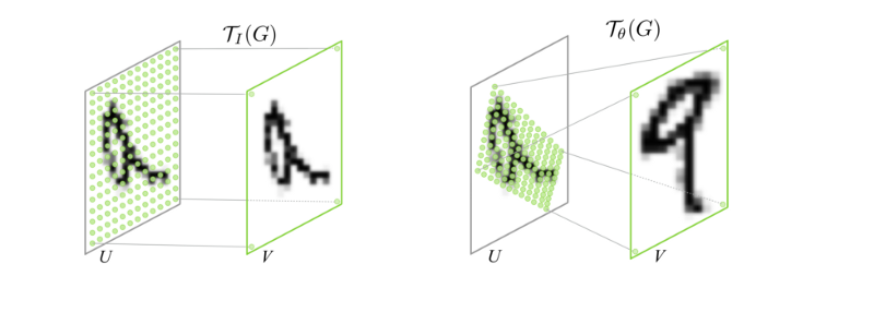
The difference here is that the sample is a single point for each neuron and it is sampling that point in a coordinate system that is the same regardless of the pooling size. That way the initialization always has something to start with.

This has two cool benefits:

1. The number of parameters is reduced from $2304+c$ to $2+mc$, where $m$ is the number of pooling steps, and $c$ is the number of channels.

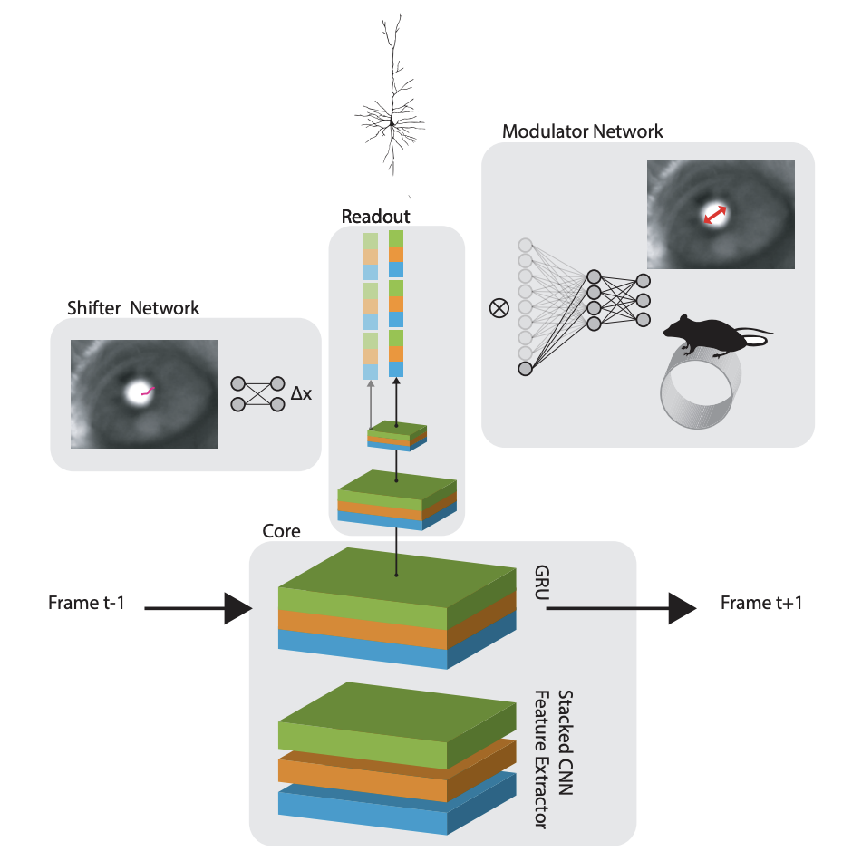
2. Eyetracking! Because the readout is parameterized as an x,y coordinate, they can shift the entire readout around with a “shifter network” that operates on the pupil position in a video of the eye.

The full model in the 2018 paper is schematized here:

Okay, so now that we have a sense of the readout, we’re ready for the new tricks introduced in Lurz et al., 2020.

New Tricks for learning the readout

Using the same bilinear interpolation readout from Sinz et al., 2018, the authors improve the learning of the $x_i,y_i$ for each neuron. They do so by using the “reparameterization trick” (Kingma and Welling)

Quick refresher on VAEs

We’ve discussed VAEs in lab meeting in the past, so we already learned the tricks that we need here to learn this new readout. This section here is a really abridged reminder on variation autoencoders with emphasis on the “reparameterization trick” as it will be applied. If you care at all about details, read (this) nice tutorial.

Start with a generative model of data $x\in {\mathbb{R}}^D$

$p(x)=\int p(x|z)p(z)dx$

where $z\in {\mathbb{R}}^{d\ll D}$ is a latent space and achieves some dimensionality reduction.

There are two tricks to learning the posterior $p(z|x)$:

First, we approximated an intractable posterior with a variational distribution $q$ and we showed that we only needed to maximize the ELBO to fit the parameters $\theta$ and $\varphi$.

Second, we reparameterized the loss to take the sampling step outsize of the optimization. This reparameterization trick let us take the gradients with respect to the parameters we’re interested in fitting. It’s the same trick they use to do the sampling here.

One final reminder about VAEs is that this is a generative modeling approach with Bayesian inference for the latents, but it can also be referred to in coding theory terms like Encoding and Decoding.

The basic idea is pictured here

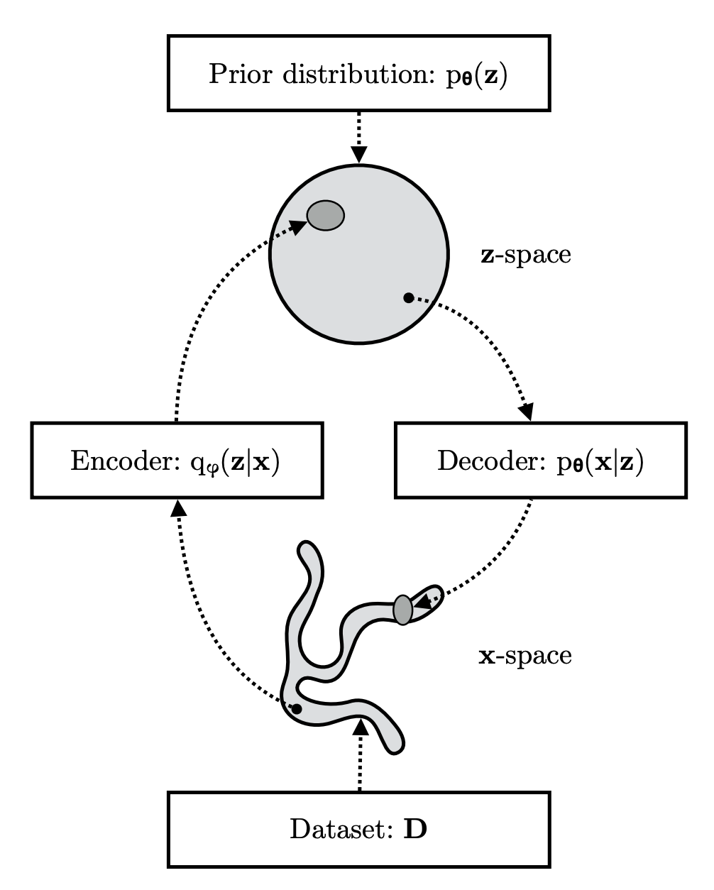
I’m going to skip derivations and you can look at the link above if you want them. The key point is that by starting with the objective of maximizing the marginal likelihood $p(x)$ you end up with two terms in the loss: one that is a KL divergence between the posterior approximation $q_{\varphi }(z|x)$ and the true (intractable) posterior $p_{\theta }(z|x)$ and another known as the Evidence Lower Bound (ELBO) that I’m showing here:

${\mathcal{L}}_{\theta ,\varphi }(\text{x})={\mathbb{E}}_{q_{\varphi }(z|x)}[\log p_{\theta }(\text{z},\text{x})-\log q_{\varphi }(\text{z}|\text{x})]$

I’m not showing the KL term here because, due to the non-negativity of the KL divergence, the ELBO is a lower bound on the log-likelihood of the data.

We want to maximize the ELBO, ${\mathcal{L}}_{\theta ,\varphi }(\text{x})$, w.r.t. the parameters $\theta$ and $\varphi$, because this approximately maximizes the marginal likelihood and minimizes the KL divergence of the approximation to the true posterior.

Maximizing the the ELBO w.r.t. $\theta$ is straightforward because the expectation is take w.r.t. the distribution $q_{\varphi }(\text{z}|\text{x})$ so we can move the gradient operator inside the expectation.

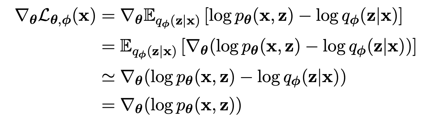
Maximizing the the ELBO w.r.t. $\varphi$ is tricky because the expectation is w.r.t. the distribution $q_{\varphi }(\text{z}|\text{x})$, which is a function of $\varphi$.

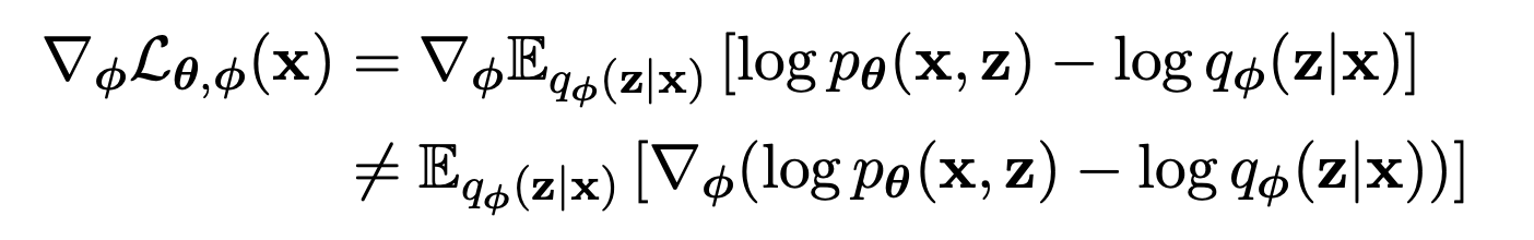
This is where the “reparameterization trick” comes in. ${\mathcal{L}}_{\theta ,\varphi }(\text{x})$ can be differentiated w.r.t. $\varphi$ with a change of variables.

First, express the random variable $z\sim q_{\varphi }(\text{z}|\text{x})$ as a differentiable and invertible transformation of another random variable $ϵ\sim \mathcal{N}(0,\text{I})$,$\varphi$, and $\text{x}$

$\text{z}=\text{g}(ϵ,\varphi ,\text{x})$

With this change of variable, the expectation can be written w.r.t. the $ϵ$ and the gradient can move inside the expectation.

${\nabla }_{\varphi }{\mathbb{E}}_{q_{\varphi }(z|x)}[f(z)]={\mathbb{E}}_{ϵ\sim \mathcal{N}(0,1)}[{\nabla }_{\varphi }f(g(\text{z},\text{x},\varphi ))]$

This reparameterization means $f(g(\text{z},\text{x},\varphi ))$ can be automatically differentiated w.r.t. the parameters $\varphi$ using whatever software is your current favorite (Tensorflow, Pytorch).

The schematic that illustrates this can be seen here:

New Trick #1: reparameterization + sampling

The model still uses the poisson loss, but now it depends on random variables $x_i,y_i\sim \mathcal{N}({\mu }_i,{\Sigma }_i)$, where ${\mu }_i,{\Sigma }_i$ are learned parameters.

The new loss function involves an expectation over the distribution of $x$ and $y$.

$\mathcal{L}(\theta ;\mathbf{r},\mathbf{x})={\mathbb{E}}_{x,y\sim \mathcal{N}(\mu ,\Sigma )}[\log p(\mathbf{r}|\mathbf{x},\theta )]$

where $\mathbf{r}$ is the observed spike counts, $\mathbf{x}$ is the stimulus, and $\theta =\varphi ,\mu ,\Sigma$ are the parameters of the model. $\mu$ and $\Sigma$ are the mean and variance of a multivariate Gaussian that generates the $x,y$ coordinates for the neuron readouts, and $\varphi$ is all other parameters in the CNN.

We can use the same reparameterization trick from above to make the gradients easy to compute. Make $x,y$ some function of a new random variable $ϵ\sim \mathcal{N}(0,\text{I})$, then the expectation is over $ϵ$ and we can move the gradient operator inside the expectation.

${\nabla }_{\theta }{\mathbb{E}}_{x,y\sim \mathcal{N}(\mu ,\Sigma )}[\log p(\mathbf{r}|\mathbf{x},\theta )]={\mathbb{E}}_{ϵ\sim \mathcal{N}(0,1)}[{\nabla }_{\theta }\log p(\mathbf{r}|\mathbf{x},\theta ,ϵ)]$

In practice, all you have to do is sample 1 draw from $ϵ\sim \mathcal{N}(0,\text{I})$ for each sample in a batch during regular old SGD.

This has a huge reduction in the number of parameters in the readout. We went from $2304\times c$ in the full space to $2304+c$ in the factorized case. Then we made it down to $2+mc$ in the coordinate + pooling case. With this final innovation, we’re down to $c+6$ parameters per neuron (not including the bias – which I didn’t include in any of the other parameter counts)!!

$c+7$ total parameters per neuron to learn for the readout should not be hard, but they don’t stop there. They use one more trick.

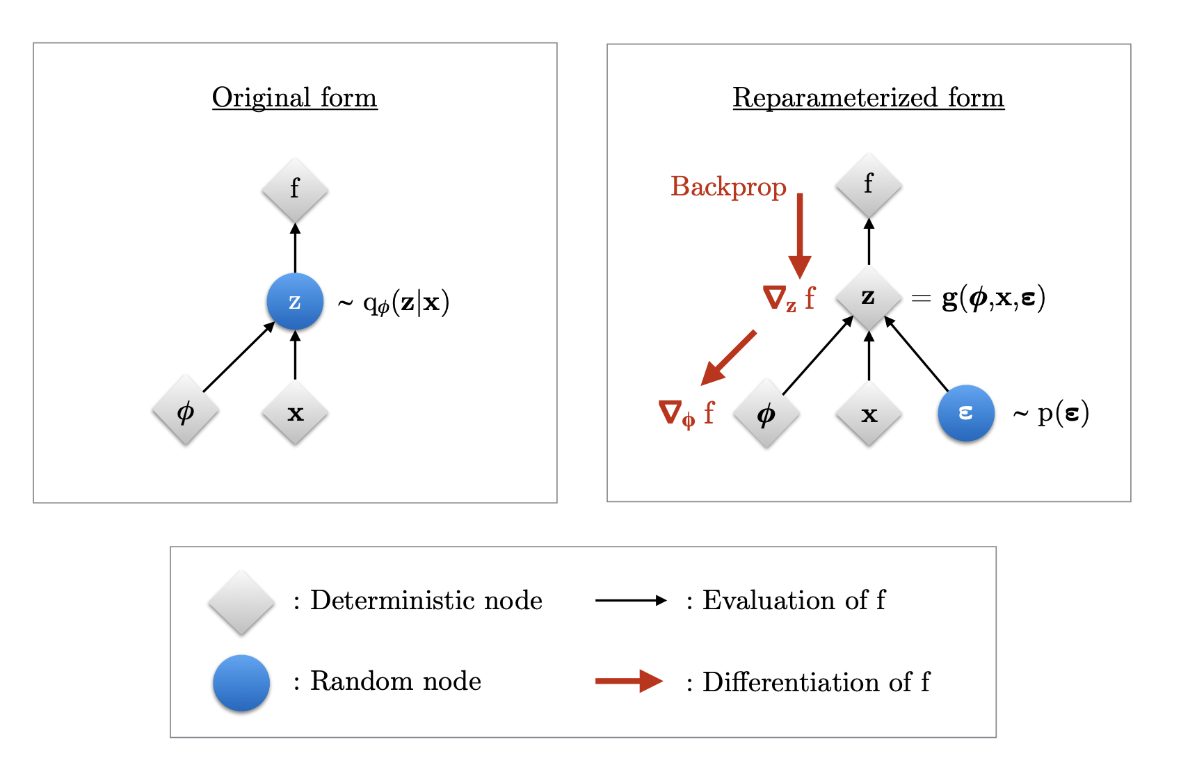
New Trick #2: retinotopy

Neurons in V1 are organized spatially such that cortical space maps onto visual space. This is known as retinotopy because cortical space forms a map that is in retinal (and therefore visual) coordinates.

Using this additional information, the authors learn a mapping from cortical space (where they measured the location of the neurons) to the $\mu$ parameter. This reduced the total number of parameters per neuron by 2 and makes shifts in $\mu$ shared.

Figure 2 in the paper illustrates this conceptually.

Now they’re really showing off! With all of these new tricks in place, they are ready to train cores and test them on withheld datasets… yea, withheld datasets, not just withheld data.

Generalization and Performance

The rest of the paper just shows how well these different readouts work for different sets of training and test data. I don’t have much to say except the new readout easily beats the state-of-the-art. And it generalizes better than VGG-16 as a core model.

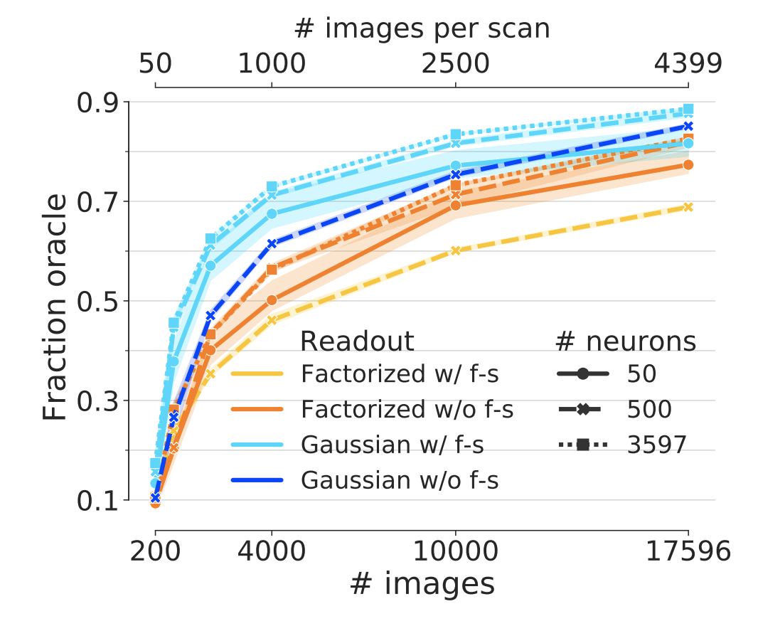
Figure 3: Performance of end-to-end trained networks. Performance for different subsets of neurons (linestyle) and number of training examples (x-axis). The same core architecture was trained for two different readouts with and without feature sharing (color) on the matched neurons of the 4-S:matched core set (Fig. 1, green). Both networks show increasing performance with number of images However, the network with the Gaussian readout achieves a higher final performance (light blue vs. orange). While the Gaussian readout profits from feature sharing (light vs. dark blue), the factorized readout is hurt by it (yellow vs. orange). Shaded areas depict 95% confidence intervals across random picks of the neuron subsets

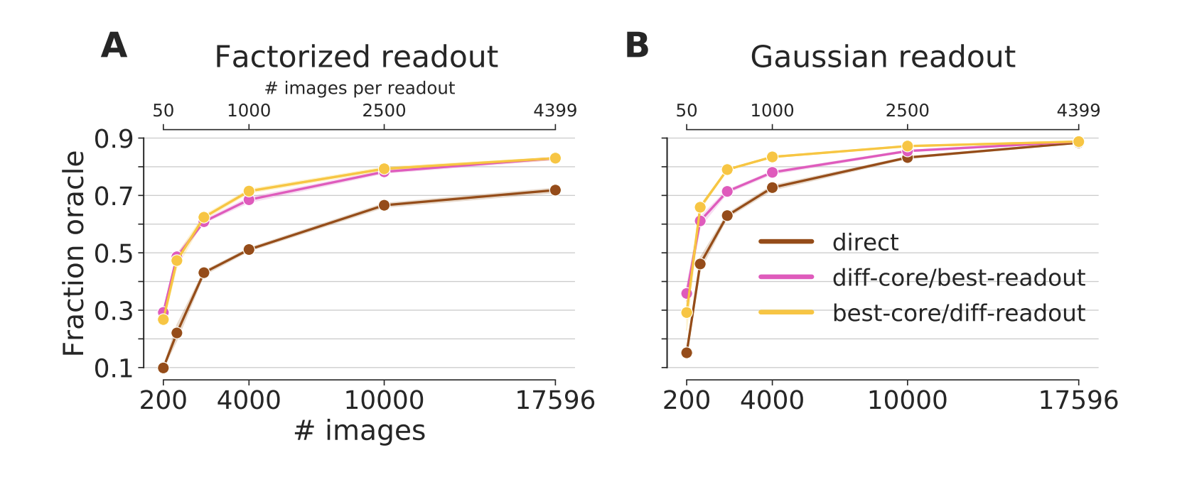
Figure 4: Generalization to other neurons in the same animal. A core trained on 3597 neurons and up to 17.5k images generalizes to new neurons (pink and yellow line). A fully trained core yields very good predictive performance even when the readout is trained on far less data (yellow). If the readout is trained with all data, even a sub-optimal core can yield a good performance (pink). Both transfer conditions outperform a network directly trained end-to-end on the transfer dataset (brown). For the full dataset, all training conditions converge to the same performance. Except in the best-core/diff-readout condition for very few training data, the Gaussian readout (B) outperforms the factorized readout (A). The data for both the training and transfer comes from the 4-S:matched dataset (Fig 1, green). Not that the different number of images can be from the core or transfer set, depending on the transfer condition.

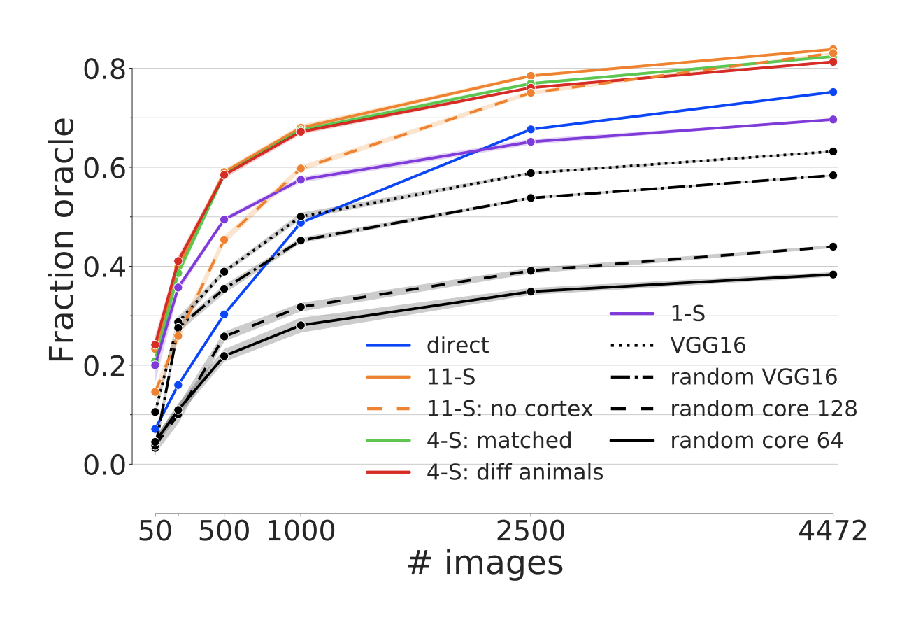
Figure 5: Generalization across animals. Prediction performance in fraction oracle correlation as a function of training examples in the transfer set for a Gaussian readout (x-axis) and different ways to obtain the core (colors). The transfer training was performed on the evaluation dataset (blue, Fig 1). Cores trained on several scans used in transfer learning outperform direct training on the transfer dataset (blue line; direct condition).

Discussion and thoughts

Overall, this is really impressive. But, I’m still left wishing these guys would do some science! Haha. Joking aside, it is nice that the ML conference format means we’re all up to date on what tricks they’re learning to fit these models, but there haven’t really been any real scientific insights from this series of papers, besides maybe the divisive normalization paper. Even the “Inception” paper was really underwhelming. All of that effort to find things that look like gabors with surrounds and don’t really drive V1 neurons much better. I’d say we’re still learning much more interesting things about mouse visual cortex using gratings, which is a real disappointment for the “state-of-the-art”. Of course, this is a high bar for a subfield that is so new, but I would be really disappointed if the ML business of focusing on performance spreads into neuroscience more than it already has. Yes, performance is important, but that alone is not the goal and performance obviously has to be mixed with insights (e.g., Kar et al., 2019) Burg et al., 2020 is definitely a step in the right direction!

I’d love to see anatomically constrained cores and attempts to explain nonlinear responses in V1 parsimoniously (like this). There are other ways this type of model could be useful. Often neuroscientists do not care about the stimulus processing model, but simply care that they have a way to modulate and predict responses so they can test for attentional modulations or decision signals. I’d like to see this framework applied to a a more natural task: the shifter and modulator networks in Sinz et al., 2018 provide a perfect vehicle to ask these types of questions.

Anyway, Lurz et al., 2020 is a very impressive method with a lot of clever tricks in it. Looking forward to the next in the series!